Statistical estimation by imitation

Parameter estimation in a subcritical percolation model with colouring, or cross-contamination rate estimation for microfluidics

We have just published a research paper ¹ about a nice combination of statistics and applied probability theory. The story opens with a novel mathematical model to quantify unwanted cross-contamination within lab-on-a-chip microfluidic devices. We apply the method of simulated moments (MSM) to estimate the parameters of the model. This method uses computer simulation with many different parameter proposals until the simulated data is close enough to the observed data. Our main contribution is that we prove the statistical consistency (`correctness’) of this method. Proving that the estimate will converge with probability 1 to the true parameter value as the sample size tends to infinity was a challenge because of the dependence among our random sample’s variables.

The motivation

While working at the Zentrum für Biosystemanalyse (ZBSA), the systems biological research insitute of the University of Freiburg, my office-neighbour Dr. Günter Roth pitched me a problem. His group develops lab-on-a-chip microfluidic devices. Theirs are 1.5 by 1.5 centimetre squared plates with more than 100,000 cavities of 19 pl volume (which is $1.9\times 10^{-11}$ litres). The cavities are arranged not in a square grid but in a honeycomb lattice (like hexagonal tiles). The value of these devices is in running many biochemical reactions in parallel, as if you had 100,000 separate test tubes. (Fun fact: one such cavity fits no more than 10,000–20,000 Escherichia coli bacteria, if you can arrange them without gaps. It’s that small.)

There is no robotic arm injecting liquid into each well (which is another name for the cavities) because it would be slow to fill them sequentially. Instead, all cavities are flooded with the same solution and it is random what kind of reaction occurs in which well. Actually, the reaction in each well is the manifold copying (amplification) of the introduced molecules. The interesting ones will be picked out by probes, which are molecules that bind to the molecules of interest but not to anything else, and the resulting signal will be strong because the target molecule has been amplified (replicated into many copies).

A concrete experiment they can do is to mix three types of DNA molecules (three different base pair sequences) and to inject this solution into the cavities of the plate. This is the so-called digital PCR (polymerase chain reaction) experiment. The DNA solution is diluted to such an extent that each cavity receives 0 or 1 DNA molecule typically, rarely more than that. This is the reason for the name digital. They run the standard PCR process to replicate the DNA molecules. For example, if they run 20 cycles, then 1 DNA molecule might give rise to 2²⁰ identical copies (minus some number due to errors in copying).

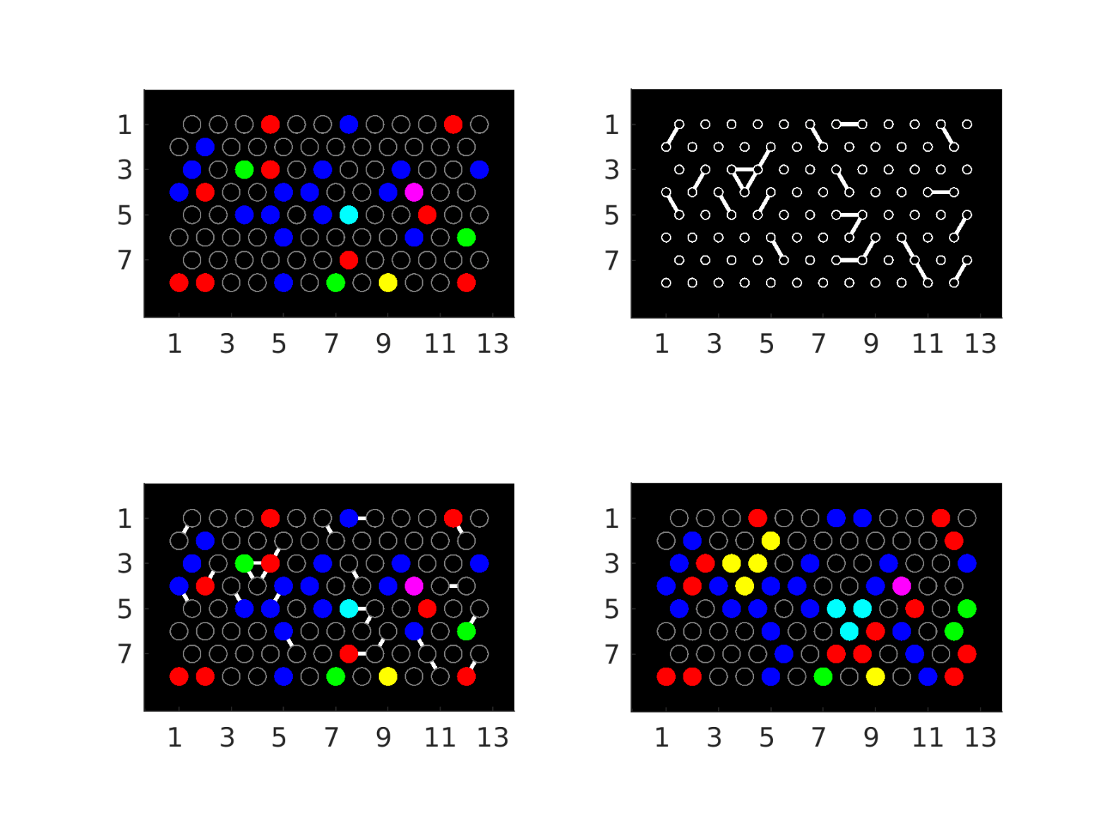
Roth’s group has also got three types of fluorescent probe molecules, one for each of the three DNA types. The first type of probes are captured by the first type of DNA and give a strong visual signal exactly where the first DNA species is located. Similarly for the second and third types. These three measurements are visualised using the three primary colours red, green and blue. We see these colours marking the cavities which originally had the DNA template of the corresponding type. The figure shows a possible observation, although this is a simulated image of a small grid. The yellow spot is red and green mixed together. (Red and blue give magenta, green and blue yield cyan, and red, green and blue together yield white.)

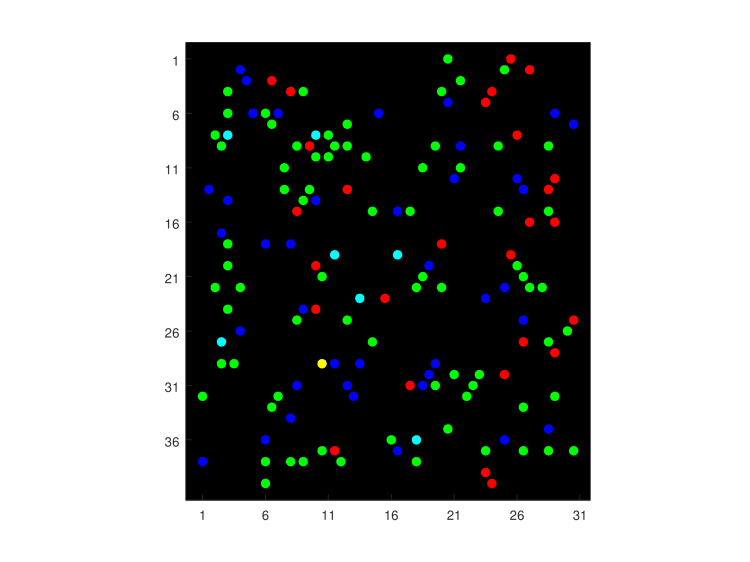
At times, they observed slides more like this. Notice the clusters of a fixed colour and the large number of spots with mixed colours (in this case, cyan). Both these patterns are suggestive of the spread of a colour into adjacent wells (concretely, of the spread of DNA copies that are later marked by a given colour). Cross-contamination combined with the encounter of another type of DNA molecules in contaminated wells is most conducive to the emergence of mixed colours.

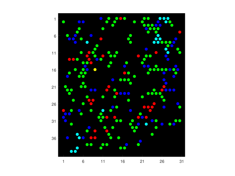
The question is, how much contamination is there in such a microfluidic chip? This is all we see, so we don’t know the initial configuration and we don’t know where DNA molecules diffused out of their original well into another one.

The model

By this point it will come as no surprise that I chose (site) percolation as the model for contamination. We have got a lattice of wells with some `communication’ between some of them. It is debatable whether it would have been better to describe cross-contamination as a unidirectional process (think of directed edges in a graph). But it just seems too hard to have random directed graphs growing from each well on the lattice in our basic model. Modelling should start with the simplest non-trivial model and percolation with its huge literature seemed like a solid foundation. It is symmetric (undirected) so that if well $i$ contaminates well $j$ , then automatically, $j$ also contaminates $i$ . This is perhaps a disadvantage of this model because this is not how the diffusion of individual DNA molecules work. But an advantage is that in percolation, one talks about clusters (components of the percolation graph). Under the model, contamination is not confined to neighbouring wells. Instead, contamination can propagate over longer distances and sweep up all wells along the way.

I decided to model the initial location of DNA molecules as being independent from the contamination process. Simply, each well has one biased coin to flip for every colour. With some unknown parameters $(\lambda^{\textrm{red}},\lambda^{\textrm{green}},\lambda^{\textrm{blue}})$ , any well will receive a positive number of DNA molecules associated with the red, green or blue probe with probability $\lambda^{\textrm{red}},\lambda^{\textrm{green}},\lambda^{\textrm{blue}}$ , respectively. We cannot and don’t try to distinguish in the original configuration between a single DNA molecule and multiple ones of the same type being in one well.

Step by step, the model can be described like this. First, we fix the seeding with DNA templates. This means that each well receives randomly the colours red, green, blue with probabilities $(\lambda^{\textrm{red}},\lambda^{\textrm{green}},\lambda^{\textrm{blue}})$ . Any well can receive multiple colours, and these choices are independent from each other (both the different colours in a single well and the seeding among different wells) (Figure, top left). Independently from the seeding, we fix a realisation of bond percolation. That is, on the triangular lattice (which is the dual of the hexagonal tiling), between any two adjacent wells, the connecting edge is included (or open) with probability $\mu$ (Figure, top right). We superimpose the two (Figure, bottom left). Finally, in the contamination step, all colours of any connected component are propagated to all wells of that component (Figure, bottom right). This results in frequent observation of the mixing of the primary colours.

The task is to estimate both contamination and seeding rates: the four parameters $(\lambda^{\textrm{red}},\lambda^{\textrm{green}},\lambda^{\textrm{blue}},\mu)$ in one fell swoop, if we observe only the last panel (Figure, bottom right). How would you do that?

Remark Some small remarks are due. First, whoever makes the DNA solution should know the concentration. Still, we don’t want to use that information because of the inherent noise in those measurements. This formulation is cleaner with four unknowns than it would be with three rather sharp distributions for the seeding rates and one unknown for the percolation parameter. Secondly, the lattice doesn’t have to be triangular, our method also works for the square lattice, and the number of colours can be anywhere from one up, it doesn’t have to be three. Thirdly, the percolation must be subcritical. This essentially means that there cannot be so many open edges that many, many wells form one large cluster. There is no point in using this microfluidic device if there is so much cross-contamination, and our proof does not work either.

The statistical method

Next, I contrast the method of our paper with the classical method of moments. There is data $\mathcal{Y}$ given, and there is a model we believe describes rather well the process which generated the data. This model has an unknown parameter vector $\theta\in\Theta$ , where $\Theta$ is typically a subset of a (potentially multidimensional) Euclidean space, and the model outputs a random variable $Y$ .

We define functions of the data, at least as many as the dimensionality of parameter $\theta$ , and usually not more than that. The coordinates of this multidimensional function $K(\mathcal{Y})$ are the moments or generalised moments (if they include something other than powers of the data). We denote the expectation of $K$ if the parameter value is $\theta$ by $k(\theta):=\mathrm{E}_\theta [K(Y)]$ .

The method of moments is the instruction to equate $K(\mathcal{Y})$ and $k(\theta)$ , and solve the equation

$K(\mathcal{Y})=k(\theta)$

for $\theta$ . The solution is the parameter estimate $\widehat{\theta}$ . Of course, this only works if we know the analytical form of $k(\theta)$ .

In our case, the obvious candidates for moments are the first moments of the colour status of single wells with a fixed primary colour. These are the means of $0$ ‒ $1$ variables (the colour is absent or present), and give three moments in our case (one each for red, green and blue). But we have four parameters, not only three, so we need some more moments.

Because we are trying to estimate $\mu$ , the rate at which insulation between wells broke down, it is natural to look at the product of the colour status of well $i$ and well $j$ for adjacent wells. This product is $1$ if and only if both wells $i$ and $j$ have the colour, $0$ otherwise. This definition yields a further three moments, one for each primary colour.

The trouble is just that it’s a hopeless task to compute these expectations analytically: the probability that a well has a colour is dependent on its seeding, on the seeding of its neighbours and on whether those are connected to it by edges, and on its second neighbours and their connections, and on its third neighbours and their connections, and so on. The method of moments has to give way to the method of simulated moments (MSM).

In the MSM, instead of computing $k(\theta)$ , we simulate it. We propose possible parameter values from $\Theta$ : $\theta_1, \theta_2, \theta_3, \dots$ . We simulate with a computer the model $n_s$ times with each of these parameters, and compute the mean of the function $K$ for each fixed parameter:

$\displaystyle\frac{1}{n_s} \sum_{s=1}^{n_s} K(Y^s)$ .

Instead of setting this equal to the observed $K(\mathcal{Y})$ , which equation we wouldn’t know how to solve, we minimise their squared difference in $\theta$ :

$\displaystyle \bigg|K(\mathcal{Y}) - \frac{1}{n_s} \sum_{s=1}^{n_s} K(Y^s)\bigg|^2\longrightarrow \mathrm{min}$

to get the estimate $\widehat{\theta}$ .

We make sure that the numbers given by the computer’s random number generator are drawn at the beginning and fixed throughout, so they are shared among our simulations of $Y$ for $\theta_1, \theta_2, \theta_3, \dots$ . This way the problem is simply a deterministic minimisation problem where if we returned to an earlier value of $\theta_l$ , we’d get the same mean for $K(Y)$ again.

Remark If you replaced the minimisation procedure with the following algorithm, then you would have an example of the popular approximate Bayesian computation (ABC) method:

Fix some $\varepsilon >0$ .

Draw random $\theta_l$ values from a probability distribution on $\Theta$ , which is called the prior distribution.
For each $\theta_l$ , generate fresh random numbers and compute $Y^s$ for $s\in\{1,\dots,n_s\}$ .
If for $\theta_l$ ,
$\displaystyle \bigg|K(\mathcal{Y}) - \frac{1}{n_s} \sum_{s=1}^{n_s} K(Y^s)\bigg|^2<\varepsilon$ ,

then accept this $\theta_l$ .

The set of all accepted $\theta_l$ is approximately the posterior distribution of the parameter value.

So what?

Although you’ve already read plenty to reach this far, the intellectual challenge hasn’t been enormous. We have a probabilistic model and we estimate its parameters by generating realisations of it with different parameter values, until a realisation imitates it sufficiently. Then we stop and accept the parameter value.

This method works quite well in practice, for lattices that are large enough, e.g. with 100,000 cavities as in the real experiment. $n_s$ doesn’t have to be larger than 10, and the larger the lattice is, the smaller it can be. My MSc student Felix Beck helped me implement the algorithm and test its performance². Our publication also includes extensive performance tests. For instance, on a $300\times 300$ grid, we can get $\mu$ with 12% accuracy. Our Matlab program is available on GitHub³.

The difficult work in the paper is to prove that this estimation procedure is strongly consistent, that is, the estimate $\widehat{\theta}$ converges almost surely to the true parameter value if the sample size tends to infinity. We do this under an unproven assumption; that the generalised moments that we chose allow for the unique identification of the parameters (no two distinct parameter vectors can give the same moments). In our defence, proving identifiability is hard for the same reason that motivated the entire paper: there are no analytical formulae for the expectations.

A subjective summary of the proof

Why it is about the law of large numbers

The idea is that we have fixed a certain number of statistics (the first and some second moments) and we are looking at the distribution of spots exclusively via these. The identifiability assumption means that the correct parameter values $(\lambda^{\textrm{red}},\lambda^{\textrm{green}},\lambda^{\textrm{blue}},\mu)$ give the correct mean of the statistics and any other choice gives different means for the statistics. The correct mean is understood as the one that we would observe if the sample size (the size of the lattice) were `infinitely large’ and fluctuations by the random realisation were negligible.

Both in the experimental setup and in our simulations, we want the empirical means to converge to the expectations of the system with the respective parameter vectors. This is the law of large numbers (LLN). We want to prove this for the strong version of LLN because then our result is also stronger (in mathematical jargon, how powerful the result is). Because only on the true parameter value does the simulation give the means that the experimental realisation gave (in the limit of very large lattice sizes), any other parameter proposal would be ruled out by its lack of convergence (as the lattice size grows) to the observed means from the experiment (when its own lattice size grows). The LLN would guarantee that the means from incorrect parameters also converge to something but that would have a different value than the means of the experimental data, and for large enough lattices, this difference would tell us that we are considering the wrong parameter vector. To make matters more complicated, we also need this convergence to be uniform over all parameter vectors, but more on that later.

I learnt the strong law of large numbers (SLLN) and its proof in my second year at university, but that standard formulation does not suffice here. Normally, you would have a sample of independent, identically distributed (i.i.d.) random variables with finite variance. (Because they are identically distributed, the variance is shared among them.) In that case, the mean of more and more realisations of these random variables converges with probability 1 to the expectation of the distribution they are from.

In our percolation model, the variance is finite because all random variables can only take the values 0 or 1. However, the spots are not independent because the possibility of cross-contamination makes them positively correlated. And they are not identically distributed either because of the effect of the boundary: wells in the middle of the grid can be contaminated from all directions even from long distances, whereas wells on the boundary can only ever be contaminated from directions towards the centre of the microfluidic chip.

Therefore the proof starts with a repetition of the proof of the strong law of large numbers via Chebyshov’s inequality. (I once heard a Russian colleague point out at a conference that Chebyshov is the correct form of the name, not the commonly used Chebyshev.) In our case, the lack of independence manifests itself in cross-correlations of the variables coming up in addition to the usual variance terms. These cross-correlations need to be bounded from above.

Percolation arguments to bound interactions

When I started this project, I was aware of how big and important an area percolation theory was within probability theory but I was completely new to the field. I thought it would be useful for my career to immerse myself in it and add it to the fields where I command a basic orientation.

The difficulty in these cases is never quite knowing how deep you have to dig to find what you need. It is often not obvious when exactly you have got all the tools at hand that you can learn from books and what is the point when you have to start thinking deeply how to creatively apply them.

It is an underappreciated aspect of mathematics that even if it is not clear how important or how generally applicable a result is when you learn it, the study material is always structured in a way that you start with the most broadly applicable knowledge and you progress towards more specialised findings and tools. My research career has proved it time and again that undergraduate pure mathematics courses convey hugely versatile findings to solve mathematical problems (that is, to prove things) even if there is no time to get practice in every field during your studies. This is a testament to our professors’ competence and professional experience and also to that of the community as a whole because mathematics courses tend to be very similar across the world.

One of the first results you read about percolation⁴ is the FKG inequality. It immediately gives that in percolation things tend to be positively correlated (more accurately: uncorrelated or positively correlated). This already took care of one side of the cross-correlations in my proof of the law of large numbers.

The counterpart to the FKG inequality is the BK inequality, which to me said that the positive correlation between wells can be bounded above by how likely it is that they are connected. We are still only in the second chapter of a standard percolation theory textbook by Geoffrey Grimmett. With an elementary but wasteful argument from as early as Chapter 1 of the book, I could make this work but only for parameter value $\mu$ below a certain threshold.

My professor recognised that if this works, then there is no reason for it not to work all the way to the critical value of $\mu$ where suddenly so many wells are connected that an infinitely large connected part starts forming. That is a qualitative change in the behaviour of the percolation graph but there is no significant change until that point.

A colleague at the University of Bristol, with more direct experience, gave me what I needed: the result is called the exponential decay of the cluster size distribution. Guess in which chapter of the book this is out of 13? It’s in Chapter 6. The result says that for subcritical $\mu$ , the probability that a fixed well $i$ is in a graph component that consists of at least $k$ connected wells decreases exponentially as $\textrm{e}^{-k g(\mu)}$ for some function $g$ . The point is not $g$ but the dependence on $k$ .

Intuitively, if you want that a direct connection of open edges exists between vertex $i$ and vertex $j$ , then if they are $k$ steps apart, then the probability is $\mu^k$ , which decreases exponentially in $k$ because $\mu <1$ . The situation is way more complicated because an open connection can take a longer, winding path. The situation is actually infinitely more complicated because there are infinitely many possible self-avoiding paths connecting $i$ and $j$ . It is the exponential decay result that captures this infinite summing in an applicable manner.

I mentioned that in addition to dependence, the identical distribution part of i.i.d. is also missing because of the boundary effect. It turned out that the effect can be quantified by estimating the probability that a well $i$ is connected via open edges to the boundary. This is determined by two factors: how many boundary wells there are and how likely is a connection from any fixed one of them to well $i$ . The second factor is once again tackled by the exponential decay of the cluster size distribution. (From which chapter?!)

I control the number of boundary wells by an explicit assumption on the lattice shape. I stipulate that the number of boundary wells divided by the total number of wells in the area of interest must tend to zero as the lattice size increases. This rules out fractal-like, rich boundaries.

It is interesting to contemplate the following moral of this result. The strong law of large numbers might work even if the random variables are not independent but their dependence is quantifiably small. The quantification in this spatial setting is the exponential decay of the probability of larger clusters of interacting random variables forming. Or to turn it around, an exponential decay of dependence is at times almost as good as independence.

The uniform version of the law of large numbers

There was still a substantial part of the proof missing. It is not enough to prove for every possible parameter vector the almost sure convergence of the mean to the expectation, the convergence also needs to be at a uniform rate across the set of possible parameter vectors. Indirectly, if there is always some small set of parameter vectors where the convergence is at a snail’s pace, then those might by chance appear to be giving a closer match to the dataset than the true parameter and trick the estimation algorithm into a wrong conclusion.

Somehow I figured it out that although probability theorists are experts of convergence questions, when it comes to uniform convergence and to the uniform law of large numbers, you have to talk to mathematical statisticians. This is because uniform convergence over the parameter set, or basically any question about a family of probability distributions indexed by a parameter (which is not time!), is by definition the realm of statistics.

At the major joint congress of probabilists and mathematical statisticians, I asked a respected statistician about my problem and they immediately referred me to the absolute expert. I found this second professor at the congress, and in one of the breaks I quickly introduced my problem. I was directed towards the method of chaining and the work of Michel Talagrand. This opinion was also supported by another colleague at a dinner who was at my seniority level. Full of confidence, back home in Freiburg I barricaded myself into the university library and started reading. Read did I about chaining, and about the theory of large deviations because it seemed to be needed for the necessary condition of chaining to work. Large deviations in themselves are as big a subject as percolation was.

Slowly my confidence started waning. I found myself again in the situation I described earlier: I didn’t know whether I should continue learning or whether I should start thinking harder because I had already covered all the tools necessary for my task. In the particular case there was also a conflict whether I can tackle the problem by using better statistical methodology or by understanding something extra about percolation. Where should I invest my time?

This is a challenge in mathematics that you only encounter at the research level. In my case, this happened long after the years of my doctoral studies. You are lucky if you can find somebody with just the right experience to see the solution to your problem. But even if you do, professors are so busy that in my experience you have to be pushy to get them think longer about your problem. In the particular case, I realised that there was a simpler statistical theorem to use and I needed a further step in percolation.

I only had to prove the Lipschitz continuity in the parameter vector of the expectations of the selected moments used in the estimator (notice again the broad applicability of a notion from undergraduate studies). For this, it was enough to modify a proof from our percolation theory textbook, still from its Chapter 2, but this time it was the next substantial argument after the FKG and BK inequalities (Russo’s formula).

In conclusion, you grind down mathematical problems by understanding everything you can about it from various angles. But often, no amount of reading can substitute for hard thinking. It comes with experience that you develop a feeling for how hard a problem is and how sophisticated tools you need to solve it. If your reading is overshooting it, realise that. The most well-intentioned help that I got at the congress put me on the wrong track and cost me perhaps two months in the library. I learnt great things about chaining and large deviations but try to put that onto your CV.

Pleasing your customer

Although now we can estimate the percolation parameter $\mu$ , it is worth keeping in mind that my collaborators had never asked for $\mu$ . They had not even known about its existence until I proposed my model! They wanted to know how much contamination there was. So we should express that in terms of $\mu$ .

I think that the best way to capture it is to estimate the number of wells whose insulation broke down, which is the sum of the component sizes for all graph components consisting of at least 2 wells. Its expectation is just about or a bit less than $6\mu$ times the total number of wells. (The details are in the paper.) This is then a quantity they can easily interpret.

Publishing challenges

This paper was rejected by several journals. It’s a combination of applied probability (percolation theory) and mathematical statistics that doesn’t excite either field. For probabilists the probabilistic methods, for statisticians the statistical methods are well known and not new. It is the combination that hasn’t been done before and there aren’t many people who would have persevered to do it. It could have worked very well as a collaboration between one expert from either field but would they have encountered this problem? Would they have been found and prodded by a biochemist? Would they have found the question interesting enough to work on?

At both journals which actually reviewed the paper (and where it was not the editor who rejected it without review), it took six months to get the referee reports. The review at the publishing journal led to another month of work to clarify details and that substantially improved the paper. One important lesson for me was to just submit the paper in the format it is in, don’t spend your time reformatting it with the journal’s template. You can do that once you have received encouraging reviews.

Annoyingly, a computational statistics journal rejected the paper by saying that it belonged to applied probability. You know, if the applied probability journals had all directed this work to computational statistics journals, then where could it have been published? Anyway, I made the accepting journal rich by paying the open access fee (the so-called article processing charge, although for a processing charge it’s very steep!) from my last postdoc fellowship. This fact, of course, must not influence the journal’s decision to accept for publication and it is communicated only after acceptance.

The research was funded by the AXA Research Fund, and a very memorable research stay where I was working on this problem was partially funded by the Engineering and Physical Sciences Research Council. I’m indebted to both.

References

¹Felix Beck and Bence Mélykúti. Parameter estimation in a subcritical percolation model with colouring. Stochastics, 91(5):657–694, 2019. doi: 10.1080/17442508.2018.1539089.

²Felix Beck. Parameter estimation in a percolation model with coloring, MSc thesis, Institute for Mathematics, University of Freiburg, Germany, 2015.

³Felix Beck and Bence Mélykúti. Parameter estimation of seeding and contamination rates on a triangular lattice using the method of simulated moments (MSM), 2017. Matlab software and Mathematica notebook.

⁴Geoffrey Grimmett. Percolation. Grundlehren der mathematischen Wissenschaften, Springer Berlin Heidelberg, 1999.