
Inflammation is the innate immune system’s response to tissue damage caused by trauma or infection. Thinking about it as the quickly receding rash after an insect bite detracts from the major antagonistic role it plays in medicine. As Baldur Tumi Baldursson of the National University Hospital of Iceland put it, `I tell my students, your work is inflammation. Practically all of internal medicine is just fighting inflammation.’
Inflammation is a complex process involving different cell types, mediator molecules and changes in the permeability of capillaries and affected tissue. This reaction has to be ramped up quickly to defend our body, but it must also be kept under strict control to prevent immune cells causing tissue damage themselves. On occasion, things go wrong and a patient is left with chronic, abnormal inflammation: inflammatory bowel disease, coeliac disease or rheumatoid arthritis are a few debilitating examples.
A mathematical model of inflammation control
These notes extend the findings of three researchers from Britain—Joanne Dunster (Reading), Helen Byrne (Oxford) and John King (Nottingham)—using control theoretical insights, and perhaps contribute a new aspect to our understanding of the problem. Their 2014 paper1 drew attention to a shift from understanding inflammation resolution as a passive process to an active, anti-inflammatory mechanism. The authors argued that the interaction of different cell types (neutrophils and macrophages) is crucial to this process. The paper expounded on three mathematical models of increasing level of detail.
The basic script of the modelled process goes like this. The scene is some generic sterile soft tissue, which suffered mechanical stress. The players are two different white blood cell types, neutrophils and macrophages, and a generic pro-inflammatory mediator, which encompasses molecules like THF-
The initiating physical damage causes a local increase in the amount of the pro-inflammatory mediator. Its higher concentration attracts neutrophils to the area. However, the active neutrophils die at a certain rate, and transform into apoptotic neutrophils. As they break down, they spill toxic load (e.g. reactive oxygen species), damaging tissue and actually increasing the level of the pro-inflammatory mediator. Macrophages accompany neutrophils in responding to the original signal, and once there, they remove apoptotic neutrophils. While neutrophils on their own prolong inflammation by the positive feedback loop, macrophages present a negative feedback loop.
Let me show the first of the paper’s three ordinary differential equation models. The concentrations of active and apoptotic neutrophil populations are denoted by 


The initial condition is 


Moreover, a bifurcation diagram indicates that an increase in the rate of macrophage phagocytosis (macrophages clearing apoptotic neutrophils) increases the likelihood of healthy resolution. Additionally, independent research had suggested that the rate of neutrophil apoptosis 
The second model, where active neutrophils release pro-inflammatory mediator
The additional assumption here is that neutrophils fight pathogens (even mistakenly, when pathogens are not present) by the release of toxins, thereby increasing levels of the pro-inflammatory mediator. After a rescaling for clarity (with the new variables and constants denoted by the original symbols), Model 2 takes the following non-dimensionalised form:
This recovers Model 1 when 


For physiologically relevant parameter values 
The conclusion from Model 2 is that for the resolution of inflammation, not only a high enough rate of phagocytosis is needed, but in my opinion counterintuitively, this should be accompanied by a rate of neutrophil apoptosis that is not too low to rule out bistability. I find this counterintuitive because neutrophil apoptosis in the short term causes a spike in the generic pro-inflammatory mediator. On the other hand, in the long run the removal of neutrophils contributes to inflammation resolution.
Some control theoretical insights in systems biology
From the viewpoint of control engineering, inflammation is an interesting phenomenon because it must exhibit rapid amplification, but it should not overshoot, requiring effective feedback control. It is natural to anticipate that this discipline can tell us something new about inflammation, and I present evidence in the following.
To me, the counterintuitive behaviour was reminiscent of non-minimum-phase dynamics. A standard example is driving a car in reverse: when we turn the steering wheel, the car turns in the direction we want to go, but not before swinging in the opposite direction2. I can recommend the whole review2 by my former postdoc supervisor Mustafa Khammash about insights in biology from robust control.
The paper 3, which preceded the review, wrote:
Control engineers make considerable efforts to avoid non-minimum phase systems, as they are generally subject to undesirable tradeoffs […] [T]he attenuation of some disturbances must come at the expense of the amplification of others. […] [I]ncreasing feedback gains, which might otherwise help with the rejection of disturbances, can lead to increasing oscillation and, ultimately, instability.
The authors Buzi, Lander and Khammash went on to argue that a simple feedback mechanism with non-minimum-phase behaviour is not robust to perturbations and is unlikely to be prevalent in stem cell differentiation. Instead, they proposed and predicted a modified differentiation feedback architecture with lineage branching, which exhibits minimum phase behaviour. They also presented possible biological examples consistent with the latter model.
It is worth highlighting here Gunter Stein’s Bode Lecture from 1989, published in 20034, as a classic on robust control and on its fundamental limitations. It is highly recommended reading.
The claim I make is that Model 2 possesses non-minimum-phase dynamics in a biologically relevant parameter regime, as I show with calculations performed with the computer algebra system Mathematica by Wolfram Research, Inc. Model 1 is a boundary case which just misses that. I do not discuss Model 3 of Dunster et al. because the calculations were too difficult even with Mathematica to reach a conclusion.
Non-minimum-phase dynamics in continuous-time linear systems
Consider a rather generic linear time-invariant (LTI) system describing the evolution of state vector 


The solution of this system is explicitly

When I studied complex analysis, one of the take-home messages ingrained in us was that whenever you see a convolution, like here from input to output, you must take its Fourier transform because that transforms it into a more tractable product. Control engineering conventionally takes the similar Laplace transform, see e.g. Section 2.6 of Reference 5.


For the special case of 

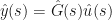

where 


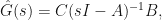
I won’t go into detail why, but the system is called minimum phase if both the roots (also called zeros) and poles of
As explained in Refs. 3 (Box 2 in Methods) and 4, Bode’s integral formulae express conservation laws about how good controllers can be at compensating disturbances. Even in an ideal case, some limit on performance cannot be surpassed. In non-minimum-phase systems, there is always some frequency where disturbances are amplified instead of rejected. This is why you can reverse with your car at low speed, but at higher speeds you’d be confused and would lose control.
Calculations in the inflammation models
In the following, I show how to compute the roots of the transfer function in Mathematica, first for the more transparent Model 1. We start by linearising the system around a steady state, so we copy the Jacobi matrix from (5)1. To follow the notation we have used so far, I denote the system matrix by

A = {{-\[Nu], 0, 0, 1}, {\[Nu], -\[Gamma]a*P, -\[Phi]*a, 0}, {0,
   0, -\[Gamma]m, 1}, {0, Q, 0, -1}}
MatrixForm[A]


MatrixForm[s*IdentityMatrix[4] - A]
sImA = Inverse[s*IdentityMatrix[4] - A]
whose entries are filled with rational functions. Now on to the choice of 

Because we are interested in the effect of changing the rate of neutrophil apoptosis ![B=[-\nu_2 \ \nu_2 \ 0 \ 0]^{\mathrm{T}}](https://s0.wp.com/latex.php?latex=B%3D%5B-%5Cnu_2+%5C++%5Cnu_2+%5C++0+%5C++0%5D%5E%7B%5Cmathrm%7BT%7D%7D&bg=ffffff&fg=111111&s=0&c=20201002)


What should be the measured quantity, how to choose 
![C=[1\ 0\ 0\ 0].](https://s0.wp.com/latex.php?latex=C%3D%5B1%5C+0%5C+0%5C+0%5D.&bg=ffffff&fg=111111&s=0&c=20201002)
![C=[0\ 0\ 0\ 1]](https://s0.wp.com/latex.php?latex=C%3D%5B0%5C+0%5C+0%5C+1%5D&bg=ffffff&fg=111111&s=0&c=20201002)
C0 = {{0, 0, 0, 1}}
B1 = Transpose[{{-\[Nu]2, \[Nu]2, 0, 0}}]
L1 = Together[C0.sImA.B1]
zeros = Solve[L1 == 0, s]
The result is 
The solution for ![C=[0\ 1\ 0\ 0]](https://s0.wp.com/latex.php?latex=C%3D%5B0%5C+1%5C+0%5C+0%5D&bg=ffffff&fg=111111&s=0&c=20201002)

![C=[0\ 0\ 1\ 0]](https://s0.wp.com/latex.php?latex=C%3D%5B0%5C+0%5C+1%5C+0%5D&bg=ffffff&fg=111111&s=0&c=20201002)

In Model 2, the calculation is more challenging. The linearisation (9b) is entered by
A = {{-\[Nu], 0, 0, 1}, {\[Nu], -\[Gamma]a*P, -\[Phi]*a, 0}, {0,
   0, -\[Gamma]m, 1}, {R, Q, 0, -1}}
MatrixForm[A]
sImA = Inverse[s*IdentityMatrix[4] - A]
B1 = Transpose[{{-\[Nu]2, \[Nu]2, 0, 0}}]
Once again, it is very hard to make use of ![C=[1\ 0\ 0\ 0],](https://s0.wp.com/latex.php?latex=C%3D%5B1%5C+0%5C+0%5C+0%5D%2C&bg=ffffff&fg=111111&s=0&c=20201002)
![C=[0\ 0\ 0\ 1]:](https://s0.wp.com/latex.php?latex=C%3D%5B0%5C+0%5C+0%5C+1%5D%3A&bg=ffffff&fg=111111&s=0&c=20201002)
C0 = {{0, 0, 0, 1}}
L1 = Together[C0.sImA.B1]
I substitute the values of 

numL1 = Collect[Numerator[L1],
   s] /. {P -> 1 + a (\[Gamma]m/\[Phi] - a)^(-1),
   Q -> 2 \[Gamma]a \[Beta]a^2 a (\[Beta]a^2 + a^2)^(-2),
   R -> (2 kn \[Beta]n^2 n) (\[Beta]n^2 + n^2)^(-2)}
to solve the equation for the zeros of the transfer function
zeros = Solve[numL1 == 0, s]
One root is 

This is a fraction with enumerator 

It helped me to use the bit of code


Collect[a^4 kn n \[Beta]n^2 + 2 a^2 kn n \[Beta]a^2 \[Beta]n^2 +
  kn n \[Beta]a^4 \[Beta]n^2 - a n^4 \[Beta]a^2 \[Gamma]a -
  2 a n^2 \[Beta]a^2 \[Beta]n^2 \[Gamma]a -
  a \[Beta]a^2 \[Beta]n^4 \[Gamma]a, a]
Collect[a^4 kn n \[Beta]n^2 + 2 a^2 kn n \[Beta]a^2 \[Beta]n^2 +
  kn n \[Beta]a^4 \[Beta]n^2, kn n \[Beta]n^2]
Collect[-n^4 \[Beta]a^2 \[Gamma]a -
  2 n^2 \[Beta]a^2 \[Beta]n^2 \[Gamma]a - \[Beta]a^2 \[Beta]n^4 \
\[Gamma]a, \[Gamma]a \[Beta]a^2 ]
to discover this. 

According to Table 41, 


Furthermore, from Figure 6, 


This was the case of ![C=[0\ 1\ 0\ 0].](https://s0.wp.com/latex.php?latex=C%3D%5B0%5C+1%5C+0%5C+0%5D.&bg=ffffff&fg=111111&s=0&c=20201002)
![C=[0\ 0\ 1\ 0],](https://s0.wp.com/latex.php?latex=C%3D%5B0%5C+0%5C+1%5C+0%5D%2C&bg=ffffff&fg=111111&s=0&c=20201002)
Conclusion
The calculations show that something is strange either with the above Model 2 of inflammation by Dunster et al., or with inflammation itself. It exhibits non-minimum-phase dynamics around the positive steady state, which is in general an unwanted property. Whether this quirk has any significant role in the development of chronic inflammation leaves me curious. Is there a frequency range where inflammation is more sensitive to disturbances, and do such disturbances actually exist? Are they relevant in any pathologies? If some of you (perhaps with more experience in control engineering) has something to add, please let me know.
(Commenting requires an email address, but it will not be publicly displayed.)
References
1Joanne L. Dunster, Helen M. Byrne, and John R. King. The resolution of inflammation: a mathematical model of neutrophil and macrophage interactions. Bulletin of Mathematical Biology, 76(8):1953–1980, 2014. doi: 10.1007/s11538-014-9987-x ($).
2Mustafa Khammash. An engineering viewpoint on biological robustness. BMC Biology, 14:22, 2016. doi: 10.1186/s12915-016-0241-x.
3Gentian Buzi, Arthur D. Lander, and Mustafa Khammash. Cell lineage branching as a strategy for proliferative control. BMC Biology, 13:13, 2015. doi: 10.1186/s12915-015-0122-8.
4Gunter Stein. Respect the unstable. IEEE Control Systems Magazine 23:12–25, 2003. doi: 10.1109/MCS.2003.1213600 ($). Free download.
5Geir E. Dullerud, Fernando G. Paganini. A course in robust control theory: a convex approach. Vol. 36. Springer-Verlag New York, 2000. doi: 10.1007/978-1-4757-3290-0.
