Santa’s Christmas delivery route revealed

Data visualisation meets children’s curiosity. We immerse ourselves in geoinformatics to find out how postal services in the USA, in Germany and in Hungary carved their countries into mosaics of postal code areas. Visually striking maps emerge from the opaque depths of numerical data.

Whoever still sends letters by post will notice that addresses closest to you share your postal code or differ only slightly, but opposite corners of your country will have very different codes. How do postal services cover countries with postal codes?

Peano curves

Let us start with a short popular science detour. If there ever were a square-shaped country, would it be possible to walk through it such that you visit every single point in that country in a single go? Can a continuous curve exist that fills the square? Continuous is a technical term of mathematics and it basically means an uninterrupted line, a curve that you can draw with a pen without lifting the pen from the paper. An abstract condition makes this task seemingly impossible: the curve must be a line in the mathematical sense, it has zero thickness. It has no width. How could such a line fill a square?

In 1890, the Italian mathematician Giuseppe Peano found such a curve, and the next year the German mathematician David Hilbert came up with a slightly simpler example. Both examples are defined through a series of ever longer curves that go closer and closer to all points of the square. Here is Hilbert’s example. He divided the square into four small squares, and connected the centres of each with a polygonal path. Each of the four squares can be subdivided into four smaller squares, and basically a shrunk version of the original polygonal path can be placed into it—the ends of these short paths will link up. And then you should repeat this subdivision of squares and the shrinking of polygonal paths forever.

Source: Wikimedia Commons, User:Braindrain0000

The actual solution curve is the limit of the finite-length curves, and its length is infinite. It is still a curve in the sense that you can map any finite interval, like , following a fixed rule to a point in the square, and the mapping will be continuous. Concretely, if you are on holiday from 25^th August until 1^st September 2018 in Squareland, there is a mapping from the time interval to the country which tells you for each moment where you have to be to complete your tour, without having to teleport from one point to another, or leave the country to enter at a different border crossing.

Next, here is the Peano curve. What you see are the first iterations, and the actual Peano curve is the limit of this iteration process. The subdivision here is always to nine small squares.

Source: Wikimedia Commons, User:Tó campos1

These curves are fractals, and a simple argument (or proof, if you’re not afraid of the term) shows that a curve to the square with the properties that it is both continuous and space-filling must visit some points multiple times. On your visit to Squareland, you will have to pass through some locations multiple times.

This subject is quite mind-boggling by all means, but it’s not the exclusive realm of geniuses. If you study mathematics at university, you may well encounter it in your first year. Enough of Peano curves: how close do postal code area planners come to this ideal solution?

Postal code area maps

We dig into data to find this out. I haven’t done any research into the planning or the evolution of this partitioning (any background info is welcome in the comments), I present only the observed state.

The source of the data for Germany and Hungary is OpenStreetMap (OSM). OpenStreetMap is a free and collaboratively built map of the world. I have become so enthusiastic about it that I created a profile and started contributing. This way you really notice how complete it is (at least in Central Europe). It’s hard to find a missing landmark. OpenStreetMap is also accessible via a neat mobile app: MAPS.ME. It’s informative, legible, fast. In MAPS.ME, you download a country or state in advance for offline navigation. If you want incremental downloading, you can use the OpenStreetMap website from your phone.

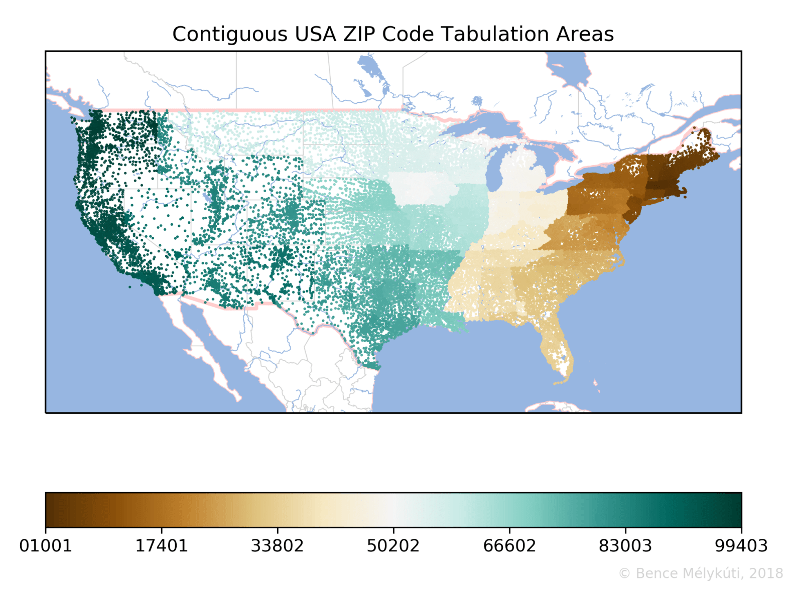
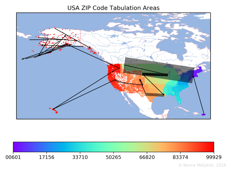
But there are only few countries whose postal code areas have been entered into OpenStreetMap. For the United States of America, I used the quasi-official source for the ZIP Code Tabulation Areas (ZCTAs) (see also this), the US Census Bureau website. The postal code areas are closed polygonal paths. I reduced these areas to single points by averaging the coordinates of the paths’ vertices. These points are displayed using colour-coding.

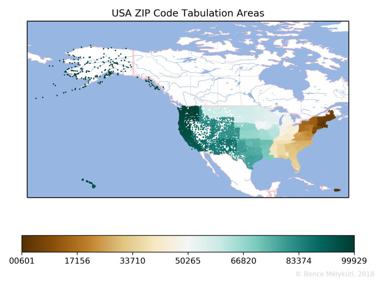
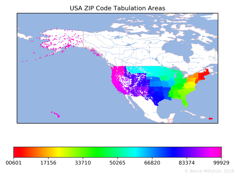
Here are the ZIP Code Tabulation Areas of the USA. The numbering starts in Puerto Rico, then progresses from the East Coast towards the West Coast, with long hops between the Pacific Northwest (Northern California, Oregon and Washington), Hawaii and Alaska.

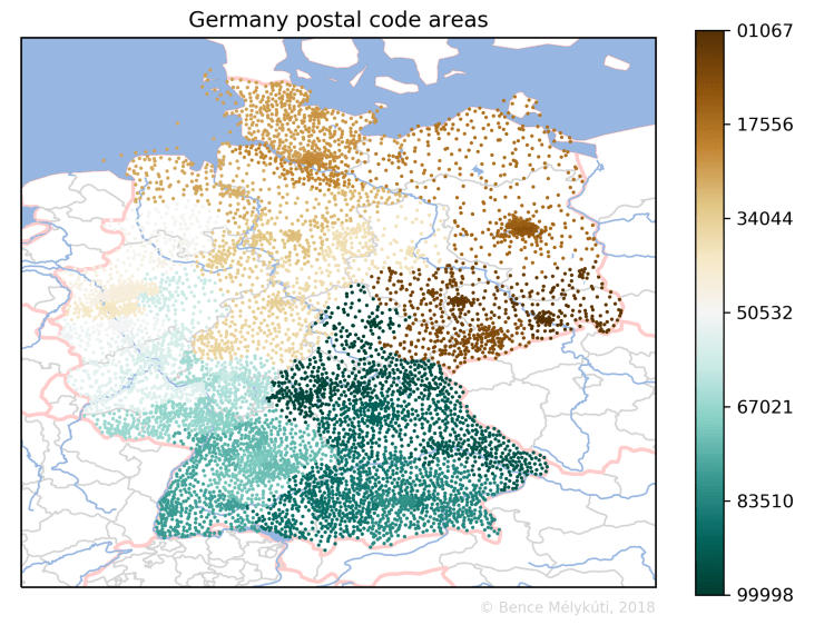
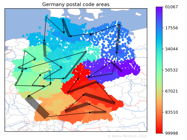
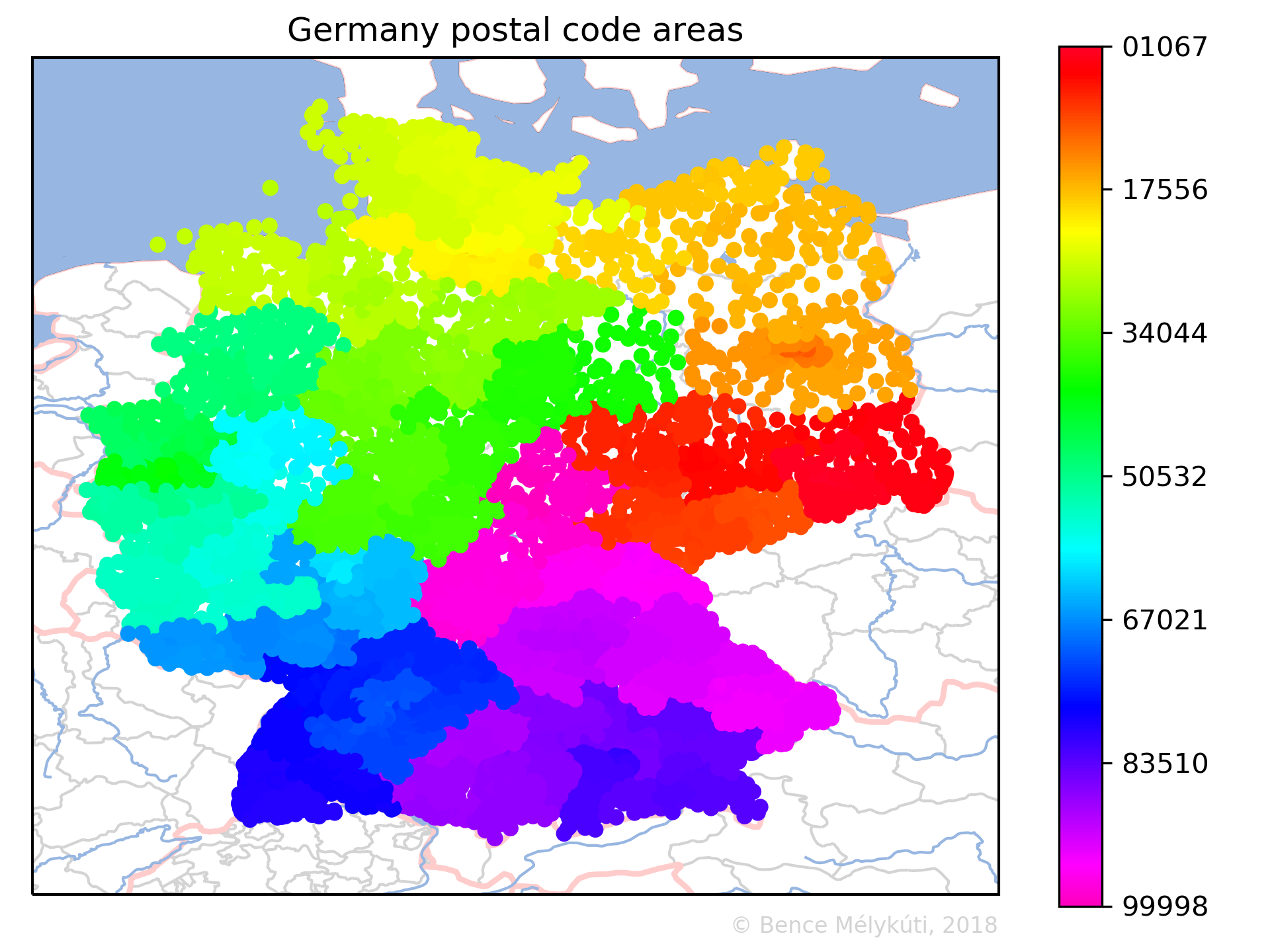
Germany uses 5-digit postal codes, but both the former East and West Germany used to have 4-digit postal codes. It would be interesting to know whether the old systems were merged in any way or a complete new system was created. How does one design such a system? Some former East German areas have numbers that start with a 0, then Berlin has numbers that start with 1.

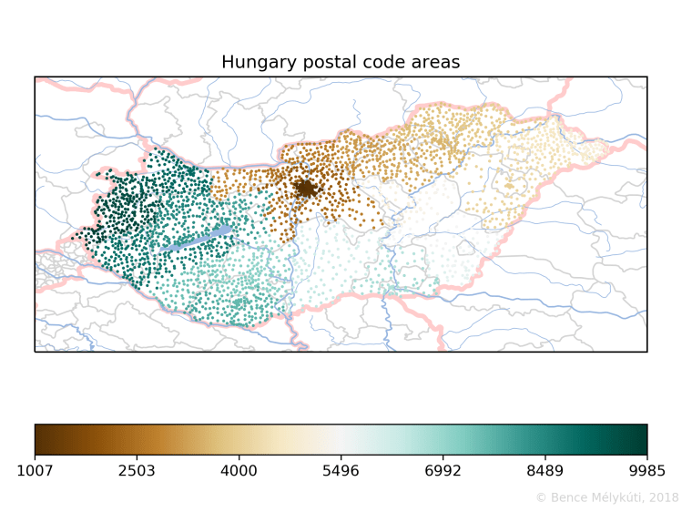
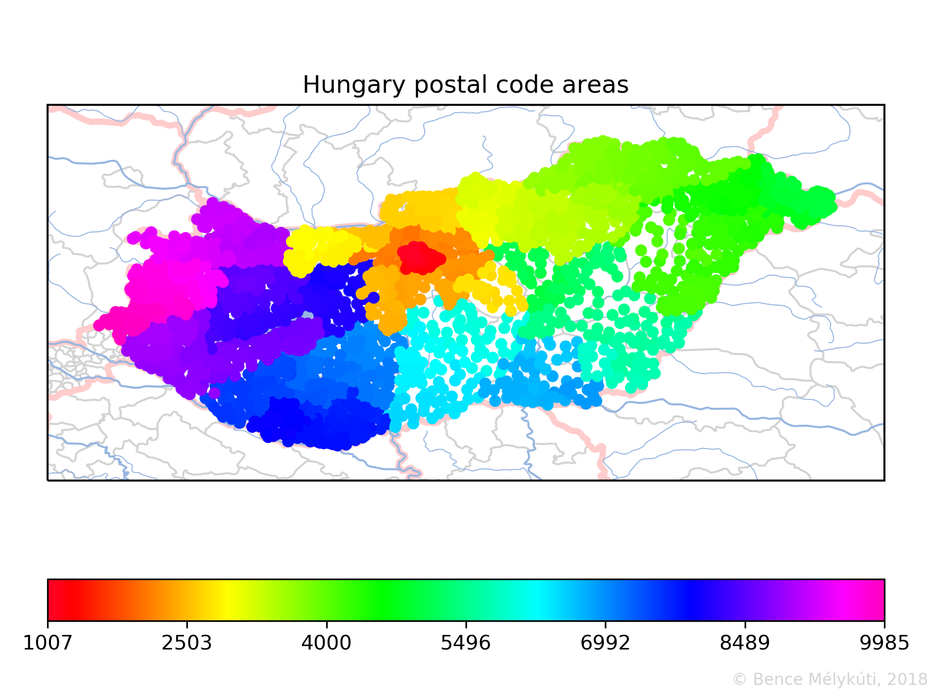
Hungary shows a nice clockwise spiralling pattern which starts in the capital Budapest. It is common knowledge that postal codes that start with 1 are the codes for Budapest. The city has 23 districts and the second and third digits of Budapest postal codes are the district number. The districts are also numbered in concentric circles broadly, in a clockwise fashion, starting from the centre. Larger organisations might have their own postal code or some postal codes might consist of post office boxes only, as far as I know. Margaret Island, the public park in Budapest with hotels and sports and leisure amenities, has postal code 1007.

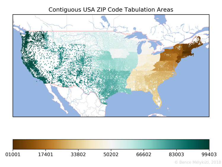
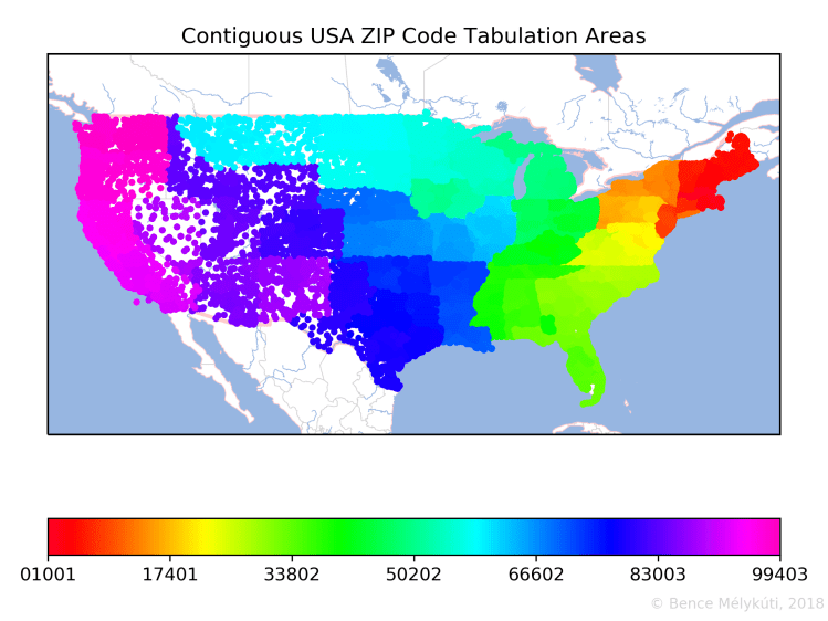
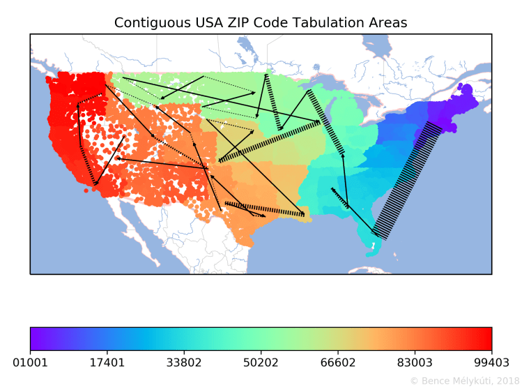
The US map already showed something interesting about population density. I assume that postal code areas are drawn in a way that each has roughly the same volume of postal traffic, which translates roughly into similar population sizes. Where postal code areas are small and the points are numerous, the population density must be high. The opposite was very visible in Alaska. (At the same time, one shouldn’t be misled by the projection that I used which might have magnified Alaska. In reality, Alaska is only four times as large as California.) By focusing on the contiguous USA and shrinking the dots, we get a better feel for postal code area density.

We can do the same with Germany. The map clearly highlights Berlin, the Hamburg area, the Ruhr region, the Stuttgart area and the Munich area as postal hotspots.

And this is Hungary with Budapest in the centre, where one fifth of the population is concentrated.

What about Santa?

If one year Santa’s sleigh is pulled by unicorns instead of reindeer, then this is how the rainbow looks like that they need to traverse to deliver all Christmas presents in the order of ZIP codes. If they leave preparations to the last minute, it would make most sense for them to start close to Santa’s home, to the North Pole, and cross the ZIP Code Tabulation Areas in descending order, from Alaska and Hawaii to Puerto Rico.

Or is it better to go from east to west, that is, in ascending order, to follow the trajectory of the Sun? That way they could deliver presents at the same local time in every time zone.

Here are the analogous maps for Germany and Hungary.

The finer structure of the designs

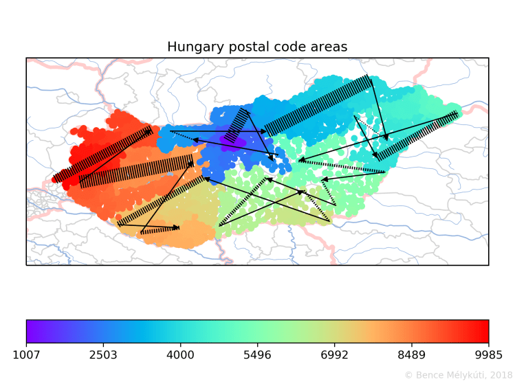
In the following, we focus on the succession of the points that mark the postal code areas. I draw solid black arrows where two successive points have a large geographical distance. These are the longest jumps, the most significant discontinuities. To help the eye find a curve, I connect consecutive arrows with transversally striped lines.

The arrows of the long jumps connect points with successive postal codes and almost identical colours. On the contrary, the striped lines are the segments where the succession of points, by drifting and diffusing, fills the space. They span ranges of colours and whole intervals of postal codes. The striped lines represent more action and are perhaps more important. They are tricky to perceive because they can be very short even if they span many, many postal code areas which might cover a large land area. For this reason, I set the width of these lines in proportion to the number of postal code areas that they span. (But again, the information is in the width of the lines, not in their width times their length, that is, the area that they cover.)

I chose a rainbow colourmap for its higher resolution than a two-tone colour scale, in a subdued tone to let the black lines dominate. We start with Hungary, which is the clearest case. The numbering starts on the Margaret Island in the heart of Budapest where the striped line starts. It ends in the west of the country.

Germany is larger but not necessarily more complicated. The numbering starts in Saxony in the east, covers Thuringia, jumps to Berlin and tackles the former East Germany before going west. It circles the country in an anticlockwise manner. The long jump in the south is to Munich.

The USA is a complete mess around Alaska with the Aleutian Islands. It is also interesting where Hawaii fits into the set of West Coast states.

On the map of the contiguous USA, it is possible to present a lot of detail about the progression of ZIP codes from east to west. There are no long jumps on the East Coast when compared to the rest of the country. The middle is covered by three east‒west corridors, of which the top two cover the Midwest.

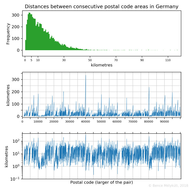
The distribution of the distances of consecutive postal code areas

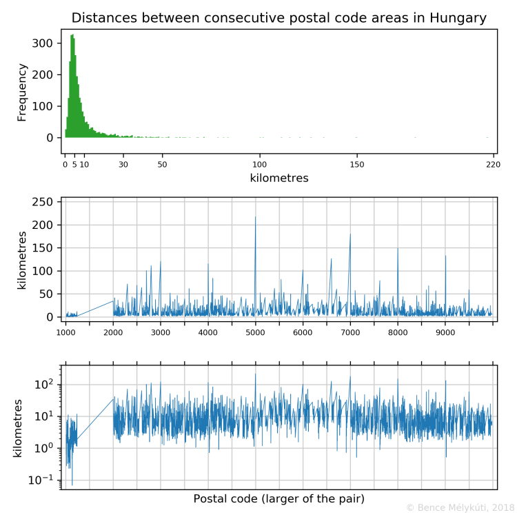
The following figures show the distribution of the distances between the computed centres of successive postal code areas via a histogram. Even adjacent areas have positive distances because I use distance between the centres of these areas. The other two plots show how large these distances are as a function of the larger of the two consecutive postal codes. They display the same data on standard and on logarithmic scales.

In the case of Hungary, larger cities, such as the seats of counties, often have round numbers as their postal code. We repeatedly see long jumps leading to round numbers. The longest jumps are to 5000 Szolnok, 7000 Sárbogárd, 8000 Székesfehérvár, 9011 Győr (from 8999), 6600 Szentes, 3000 Hatvan, 4002 Debrecen (from 3999), 2800 Tatabánya, 6000 Kecskemét, 2700 Cegléd. (I used the Hungarian Post’s postal code search web service.) This suggests that larger areas (such as counties) are frequently numbered starting from the large town, progressing outwards.

I found the shortest distance between centres of consecutive Hungarian postal code areas in Újlipótváros, Budapest, between the interleaving areas 1136 and 1137. The ten shortest distances in the country are all in Budapest, in the densely populated districts I., IV., VI., VII., VIII., IX. and XIII. They measure 200 to 500 metres.

In Germany, the longest jumps arrive at 40210 Düsseldorf (from 39649), 80331 München (from 79879), 26121 Oldenburg (from 25999), 95028 Hof (Saale) (from 94579), 10115 Berlin-Mitte (from 09669), 50126 Bergheim (from 49849), 90402 Nürnberg (from 89619), 07318 Saalfeld/Saale (from 06925), 19053 Schwerin (Mecklenburg) (from 18609), 55116 Mainz (from 54689). Frankfurt am Main, with postal codes 60306 and greater, is at the end of a jump from 59969. (Here is the Deutsche Post’s postal code search.)

Banks and other corporations have some of the postal codes of these large cities. At times these postal codes are between the preceding round number and the first geographically assigned postal code. The shortest distances between the computed centres of consecutive postal code areas are 200–500 metres, and I found them in Essen, Frankfurt am Main, Augsburg, Düsseldorf.

The US Postal Service Zip Code lookup facility helps us interpret jumps in the USA. The longest two are from Hawaii to 97001 Antelope, Oregon and from Truckee, California to 96701 in Hawaii. Next on the list is the one from 00987 Carolina, Puerto Rico to 01001 Agawam, Massachusetts, then the jump from 99403 Clarkston, Washington to 99501 Anchorage, Alaska. Then we’ve got one in the contiguous USA from 59937 Whitefish, Montana to 60002 Antioch, Illinois. Thereafter comes one within Alaska, followed by 69367 Whitney, Nebraska to 70001 Metairie, Louisiana.

I find it interesting that by the time the US Postal Service has covered Texas, all codes until 79942 have been used up. This is 80% of the codes, which seems a little wasteful! The next town is 80002 Arvada, Colorado. (At present, it also has the ZIP Code 80001. It appears that this had not yet been the case at the Census in 2010.) On second thoughts, I can’t rule out that 80% of the US population has actually been covered by Texas. California has 12% of the total US population and the populations of the remaining handful of states are quite small.

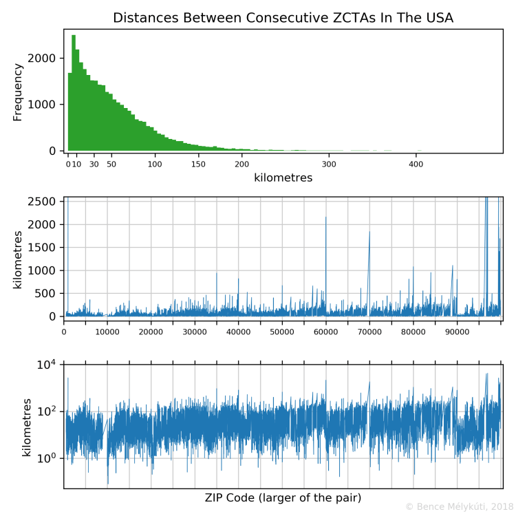
The absolute shortest distance is between two New York City codes, 10171 and 10172, at 80 metres. NYC has two more pairs with approximately 200 metres distance. Saint Louis MO, Denver CO, government bureaus in Washington DC, Shelter Island and Shelter Island Heights NY, Northfield VT and Northfield Falls VT, Charlotte NC, Chicago IL, Montgomery AL give examples for pairs of ZCTA centres only 200–300 metres apart.

These were the last figures about the postal codes and I thank the casual readers for reading this far. The following is some sort of an appendix where I discuss some of the technical aspects of producing these maps.

Things I learnt during the making of

OpenStreetMap

I want to continue singing the praises of OpenStreetMap. OSM is actually not simply the map you see on the web, it is primarily the database with all the information that may or may not be rendered on that map. You can retrieve data directly from the underlying database using its query language and display it in a graphical user interface, Overpass Turbo. Or you can retrieve very specific subsets of raw data from OpenStreetMap for processing by the Overpass API.

OpenStreetMap has an extensive wiki site. It is of great help to understand all the data labels for querying and editing OpenStreetMap. For instance, the Overpass API query language guide is extremely useful for geoinformatics projects like this one. OpenStreetMap can motivate you to discover your surroundings. You can go hunt bunkers in the beautiful hills and forests of Budapest or magnolia trees in Freiburg im Breisgau. You can query all the restaurants and pubs in an area with outdoor seating, or you can find the public toilets at your destination.

The importance of the right algorithm

These days there is much talk about cloud computing, which is the possibility to rent computer resources from enormous pools instead of buying them. This way you can access much computer power when you need it. If you need high performance only for temporary bursts but not round the clock, then it’s more economical to rent than to buy it.

It still remains important to choose the right algorithm though, instead of spending your way out of a time-consuming computation. That’s how I went from 2 h 20 min running time to 8 sec.

We have to return to OpenStreetMap briefly. The elements of geographical data stored in it belong to one of three categories: nodes, which are points on the map, ways, which are sequences of nodes which form a polygonal path, and relations, which are sets of nodes and ways and possibly of other relations. A way can be a closed path (a polygon), in which case it defines an area, like the postal code areas.

In reality, postal code areas are stored as collections of ways (that is, as relations) because the perimeter would be impractically long for a single way. Therefore I wrote a script to collect all ways for every postal code area and store them; and to collect all nodes for every way and store them with their geographic coordinates. So I had a list of all nodes (without repetition) that have been found in any way that belonged to the outer boundary of some postal code area. From OpenStreetMap, I also had the coordinates of these nodes in a tree-like data structure.

What the unsuspecting programmer does in this case is that you go through all nodes in the list, find the same node in the tree, and read out its coordinates for storing. But something was wrong: the whole dataset for Hungary I downloaded was 24.9 MB and the script ran for 2 h 20 min—no matter what you do to 24.9 MB of data, it mustn’t take that long.

The problem is, of course, that this implementation is an algorithm where is the number of nodes. For every node, I searched through potentially the whole tree. It takes on average lookups to find what you are looking for.

The right way of doing this is to accelerate the search by ordering the nodes in the tree. I used a sorted dictionary where the keys were the node identifiers and the values were the nodes with their geographical coordinates. This way, finding the node takes time, reducing algorithmic complexity to . The running time decreased a thousandfold to 8 sec.

The dataset for Hungary consists of over 222,000 nodes. It was only by the smarter algorithm that I could process the 2,734,000 nodes that the Germany dataset had. But then it took only 80 sec running time.

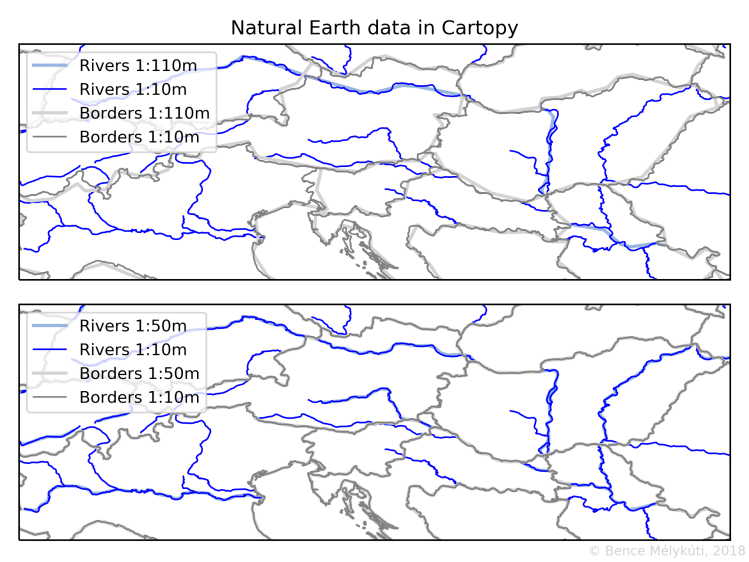
Something about Cartopy

I used the Cartopy Python package to plot my maps. Through an interface, you can easily load Natural Earth data to include e.g. country borders and natural features (coastlines, rivers, lakes) in your maps. There is a choice between scales of 1:10,000,000, 1:50,000,000 and 1:110,000,000.

For Hungary, I carelessly loaded these features at the 1:110m scale. When I plotted my spots on the map, they formed lines nicely along the state border but they were visibly off. It appeared that there was some systematic error between borders from Natural Earth and my points. The same happened with the river Danube: instead of splitting Budapest down the middle into Buda and Pest, it only skirted the capital.

Cartopy has a whole tutorial about such misalignment issues. I wasted much time on that until I concluded that my issues were gone once I imported the maps at 1:10m scale! (The below test shows that 1:50m would have been fine, too.) Smaller scale means coarser resolution, and locally this can result in errors that seem to be biased in one direction when actually the error is unbiased.

Here is a demonstration. Look how the coarser, 1:110m Danube in Budapest is off from its finer, 1:10m rendering. Similarly, in the east of Hungary, the finer state border is consistently to the east of the coarser border. In the lower panel in the comparison between 1:50m and 1:10m, everything lines up fine.

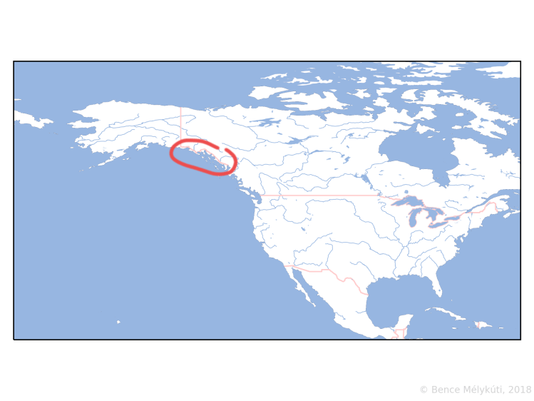
Something about Alaska

I hadn’t known that this bit of the Pacific Coast belonged to Alaska (and the USA) and not to Canada! It’s called Southeast Alaska or the Alaska Panhandle.

Update (T+8 days):

A Reddit user has kindly advised me that the German Wikipedia has the full story of the evolution of the German postal code system over different eras and of the current system as well. It was introduced after the reunification in 1993.

The first digit out of five denotes the zone. The numbering starts from the centre of the country, heads towards the south and goes around in anticlockwise direction.

Source: Wikipedia, Deutsche Post

The second digit out of five denotes the region within the zone. The numbering typically starts from the centre of the zone, heads towards the south and goes around in anticlockwise direction. It is much clearer here than on my maps. See also the very detailed list of the regions that correspond to the first two digits.

Source: Wikimedia Commons, Stefan Kühn

In the next step of the hierarchy, the region’s different towns and settlements get postal code intervals, starting with the postal centre of the region. Within these intervals, postal codes for post office boxes are followed by those for receivers of large volumes of postal traffic (e.g. local authorities, universities, administrative offices, television channels, corporations) and finally come the postal delivery areas. My maps show only this third type.

What is new about Hungary on Wikipedia is that county seats have always got numbers that end in two zeros but they are not the only towns to have such numbers. In general, towns tend to have numbers that end in a zero.